
Figure 1. Teradata in-database analytics functions for feature engineering and results.
Feature engineering is a critical step in predictive analytics, machine learning (ML), and artificial intelligence (AI) tasks. A feature is a measurable attribute in a dataset that could be reasonably deemed to be an independent variable that influences the value of the dependent variable we are modeling. For instance, to forecast home prices, relevant features might include the home’s age, size, and energy-efficiency rating. The home price is a dependent variable called a target in this scenario.
Some features might be found directly in the dataset. Others might need to be built from existing features by transforming, modifying, rescaling, or combining them. The process of selecting features with predictive value and building new features from existing ones is called feature engineering.
Feature engineering occurs after the data cleaning and exploration steps of the data preparation process, just before the training process. However, data preparation steps are usually iterative and can happen in tandem with each other.
Teradata VantageCloud’s ClearScape Analytics™ takes full advantage of Teradata's architecture. These powerful, open, and connected AI/ML capabilities include powerful in-database analytics functions that make performing feature engineering at scale a very straightforward process.
In this article, we’ll cover the usage of a set of these functions to build features relevant for a regression analysis in a customer churn dataset. The features created and functions used in this article are purely illustrative. The process of selecting appropriate methods and functions for feature engineering is a complex subject, and much falls outside the scope of this article.
Prerequisites
To replicate the practical steps outlined in this article, you'll need the following prerequisites:
- A Teradata VantageCloud instance
- A database client for transmitting SQL statements
- The customer churn sample dataset uploaded to a table in your Teradata VantageCloud instance
Obtain a Teradata VantageCloud instance
The ClearScape Analytics Experience is the most convenient way to experience Teradata VantageCloud, and it’s free:
- Set up your free ClearScape Analytics Experience account.
- Log in and create an environment. Remember your password, as it's required to connect to the database server using your preferred database client.
- Link your Teradata VantageCloud environment to your chosen database client. Any client that supports Teradata would work.
- The user is `demo_user` for all environments.
- The password is the password established while setting up the environment.
Loading dataset
The customer churn dataset sample is available as a CSV in Google’s cloud storage. We will use Teradata’s Native Object Storage (NOS) functionality to load the sample data to the database.
- First, we need to create the database by running the following script in our database client.
CREATE DATABASE analytics_features_demo

AS PERMANENT = 110e6;
- Then we need to load the data to a table by running the corresponding script
CREATE TABLE analytics_features_demo.churn_data_set AS

(

SELECT

user_id,

subs_type,

subs_start,

subs_end,

subs_length,

churn,

freq_usage_month,

usage_session

FROM(

LOCATION='/gs/storage.googleapis.com/clearscape_analytics_demo_data/DEMO_AIBlogSeries/churn_prediction_dataset.csv') as churn

) WITH DATA;
Exploring the dataset
Let’s look at the first 20 records of data ordered by `user_id`.
SELECT TOP 20 * FROM analytics_features_demo.churn_data_set

ORDER BY user_id;
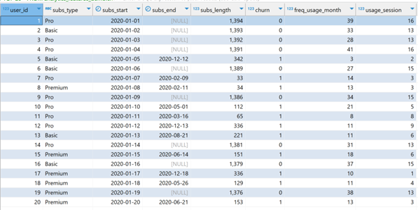
Figure 2. First 20 records in the dataset.
The exploration has revealed the data shown in figure 2. We aim to model customer churn with the following data:
- User identifier
- Subscription type
- Subscription start and end dates
- Only churned customers have an end-of-subscription date
- Subscription length
- This value is measured in a number of days, whether the user has churned or not
- Frequency of usage per month
- Average usage time (minutes per session)
Feature engineering for better predictions
Regarding the data we have, there are several features that might help us predict churn. For example, if we filter our data by `subscription type`, we may uncover patterns that indicate that certain kinds of subscriptions may churn more often. We can also explore `subscription length` to try to identify time periods during the subscriptions duration when customers are more likely to discontinue service. These features can give us insights beyond typical indicators of churn, such as, `frequency of usage per month` and `average session time`, which are often good predictors of people abandoning subscriptions.
We can directly use numerical features like `subscription length`, `frequency of usage`, and `average session time` to model a regression. However, `subscription type` is categorical, and must be encoded into ordinal values for predictive modeling, such as 1 to 3 standing for Basic, Pro, and Premium types.
Additionally, it's important to consider the scale of our features. In our scenario, we're dealing with various scales, such as the following:
- Subscription lengths measured in days, often on a scale of thousands
- Usage frequency per month measured in sessions, typically on a scale of 1 to 60
- Session lengths, typically ranging from 1 to 30 minutes
To maintain modeling efficiency and accuracy, it's crucial to adjust these scales. Without normalization, the extensive range of subscription lengths might overshadow other features. We intend to equalize all feature scales to similar levels, and fortunately, Teradata simplifies this process with its straightforward functions.
Creating new columns for encoded subscription types, and the statistical normalization of features to a similar scale exemplifies typical feature engineering steps. Teradata’s in-database analytics functions facilitate this process, allowing straightforward feature creation without transferring data to a pandas DataFrame, which might introduce inconsistencies in the data and can be time-consuming or impractical when done at scale. These functions are also easy to read and write because they don’t require complex SQL queries. Teradata analytics functions elegantly abstract the complexity.
Encoding categorical data to numbers
Teradata’s analytics functions used to perform data transformation usually come in pairs. In this function pair, the first “fits” the data by analyzing and understanding its structure, creating a table that describes the data. The second function then performs the transformation, applying the parameters determined during the fitting process.
In the case of numerical encoding of categorical data, and especially in the case of a subscription type, which is an ordinal set of categories, ‘basic’, ‘pro’, and ‘premium’, the functions `TD_OrdinalEncodingFit` and `TD_OrdinalEncodingTransform` are ideal. They encode the categories into a set of ordinal values, in this case, a range from 1 to 3.
First, we’ll apply `TD_OrdinalEncodingFit` to the dataset, as shown in the following code sample. This will result in the table shown in figure 3. This table will then be used as the dimensional input for `TD_OrdinalEncodingTransform`.
CREATE TABLE analytics_features_demo.ordinal_encoding_type AS (

SELECT * FROM TD_OrdinalEncodingFit (

ON analytics_features_demo.churn_data_set AS InputTable

USING

TargetColumn ('subs_type')

Approach ('LIST')

Categories ('Basic','Pro','Premium')

OrdinalValues (1, 2,3)

) AS dt

)WITH DATA;


SELECT * FROM analytics_features_demo.ordinal_encoding_type;
In this code, we pass as input table the churn dataset, we set the target column as the subscription type and provide the categories and the ordinal values. The result is the following table with encoded categories.
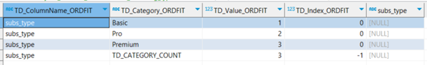
Figure 3. Subscription types encoded by Teradata `TD_OrdinalEncodingFit` function.
The fit tables resulting from applying fit functions are often persisted as tables to avoid recalculations. These tables can then be reused by other processes, or in conjunction with the `TD_ColumnTransform` function, to expedite the transformation of the same or related datasets in the future. We will see this in action when we implement the statistical normalization of features to change their scale.
Once the data is fitted, we can utilize `TD_OrdinalEncodingTransform` for a seamless transformation. In the following code block, the churn dataset is the input table, and the table with the fitted data is the `FitTable` Dimension. We `accumulate` based on the columns that we intend to keep for our modeling, this in short means that the columns mentioned in `accumulate` will be part of the result of the transformation. We persist the result as a table as it will be the base for future transformations. We kept the column `user_id` for illustration purposes. In a real scenario, we would have only kept our target, ‘churn’, and the relevant features.
CREATE TABLE analytics_features_demo.predicting_features AS (

SELECT * FROM TD_OrdinalEncodingTransform (

ON analytics_features_demo.churn_data_set AS InputTable

ON analytics_features_demo.ordinal_encoding_type AS FitTable Dimension

USING

ACCUMULATE ('user_id','subs_length','churn','freq_usage_month','usage_session')

) AS dt

)WITH DATA;


SELECT * FROM analytics_features_demo.predicting_features

ORDER BY user_id;
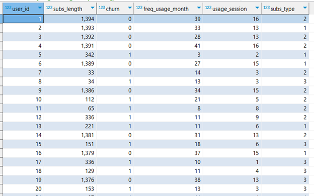
Figure 4. Features with encoded subscription types computed by Teradata `TD_OrdinalEncodingTransform` function.
It's worth mentioning that there are alternative methods for categorical data encoding. For high-cardinality categories, defined as having a high number of categories, the `TD_TargetEncoding` function family is a suitable option. On the other hand, `TD_OneHotEncoding` is beneficial for low-cardinality categories without any ordinal relationship. Additionally, the inverse process, encoding numerical values as categories through binning, is achievable with the `TD_BinCode` function family.
Normalizing the scale of a feature
Though features being on a similar scale is only a hard requirement of certain modeling techniques (specifically those based on clustering), in our case, this scale normalization might be a good idea, though it is not necessarily required for finding a regression.
The duration of a subscription is calculated in days. For long-standing subscribers, this can total into the thousands. In contrast, other metrics, such as those measured sessions or minutes, often have values in the double digits. This discrepancy could undermine the reliability of our modeling. In regression analysis, for instance, the model might overly emphasize subscription length as the primary predictor of churn. This may overshadow the predictive significance of other variables.
For the aforementioned reasons, we will normalize all the features to a scale ranging from 0 to 1. To do this, we will use the `TD_ScaleFit` and `TD_ColumnTransformer`. First, we’ll fit the data using the `TD_ScaleFit` function. This function can take several columns of the same table simplifying the entire process.
First, we need to specify the following parameters:
- Input table
- Scaling method
In the following code sample, we chose `Range` for our scaling method. By default, `Range` scales values from 0 to 1, which is suitable for this case. Although `TD_ScaleFit` offers additional parameters and scaling methods to perform further adjustments, these advanced options are beyond the scope of this discussion.
CREATE TABLE analytics_features_demo.scaled_dimensions AS (

SELECT * FROM TD_ScaleFit (

ON analytics_features_demo.predicting_features AS InputTable

USING

TargetColumns ('subs_length','subs_type','freq_usage_month','usage_session')

ScaleMethod ('RANGE')

) AS t

)WITH DATA;


SELECT * FROM analytics_features_demo.scaled_dimensions;
The previous code will generate a table that contains the results of the fitting process, the `FitTable`, which we will pass as a parameter when calling the `TD_ColumnTransformer` function later on. The results of the fitting include the following statistical descriptions of the data:
- Maximum and minimum values
- Number of records
- The scale
- This is defined as the difference between the maximum and minimum values
- The sum of the column’s values
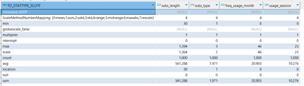
Figure 5. Fit table computed by Teradata `TD_ScaleFit` function.
Now that our data is properly fitted, we can utilize the `TD_ColumnTransformer` function. We’re opting for `TD_ColumnTransformer` (over `TD_ScaleTransform`) because of its unique capability to facilitate multiple transformations in a single step—and still retain all of the columns from our input table.
- We set the `predicting_features` table as the input table
- We set the `scaled_dimensions` as the fit table dimension
CREATE TABLE analytics_features_demo.predicting_features_scaled AS (

SELECT * FROM TD_ColumnTransformer(

ON analytics_features_demo.predicting_features AS InputTable

ON analytics_features_demo.scaled_dimensions AS ScaleFitTable DIMENSION

)as dt

) WITH DATA;


SELECT * FROM analytics_features_demo.predicting_features_scaled

ORDER BY user_id;
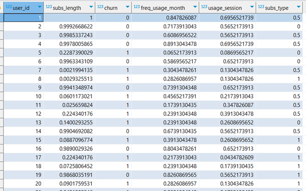
Figure 6. Features scaled to a range from 0 to 1 as computed by Teradata `TD_ColumnTransformer` function.
The regression model: Putting it all together
With the features properly scaled, we can proceed to train a model for prediction. Due to the scope of this article, we won’t cover the scoring of the model (model operationalization will be covered in future entries), thus, we are not performing a test/train split.
We will input our data into the Teradata Generalized Linear Model, `TD_GML`, which supports binary classification across multiple variables. A simple implementation of `TD_GML` will meet our needs.
As input columns we define our features: `subs_length`, `subs_type`, `freq_usage_month`, and `usage_session`. The response column is our target, `churn`. The type we set as binomial classification because we are trying to predict the odds of `churn` being 0 or 1, according to the value of the features. The intercept is set to true (the model will predict baseline odds for churn when the value of the features is 0).
The parameters `Tolerance` and `MaxIterNumber` are related. The former is the minimum improvement in prediction accuracy that the model will try to reach before stopping to iterate, while the latter signals the maximum number of iterations allowed. In summary, the model will stop training whichever happens first. If the model stops before reaching the tolerance threshold, meaning it didn’t get to predict as accurately as defined, the results will state that the model did not converge.
Note: You need both a breadth of expertise across your business field and a strong domain knowledge within data science to develop a successful strategy for predictive accuracy. Both are required to determine appropriate values and necessary iterations. This is a topic that goes beyond the scope of this article.
CREATE TABLE analytics_features_demo.GLM_model AS (

SELECT * FROM td_glm (

ON analytics_features_demo.predicting_features_scaled AS InputTable

USING

InputColumns('subs_length','subs_type','freq_usage_month','usage_session')

ResponseColumn('churn')

Family ('Binomial')

MaxIterNum (300)

Tolerance (0.0001)

Intercept ('true')

) AS dt

)WITH DATA;


SELECT * FROM analytics_features_demo.GLM_model;
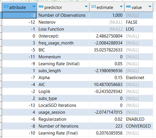
Figure 7. Results of the general regression model computed by Teradata `TD_GML` function.
The results shown in figure 7 demonstrate that the model reached the expected predictive accuracy after 223 iterations. It found that frequency of usage per month, subscription length, and session time are negatively correlated with the probability of churning. This can be seen on the negative estimate contribution to the odds of churning assigned to those features. Subscription type is irrelevant for predicting churning—its contribution to the odds of churning is 0.
As mentioned, we could use this prediction model for scoring other data points, and that would enable us to tackle the risk of profitable accounts churning before they are lost. As mentioned, model operationalization goes beyond the scope of the present article, but we will cover it in future deliveries.
Conclusions
Feature engineering involves identifying and selecting data features with predictive potential as inputs for predictive models. This process also includes modifying these features, when necessary, to align with the requirements of the chosen modeling technique. These transformations can be intricate, and they typically require extensive SQL operations—or even risky data transfers to pandas DataFrames. Teradata's in-database analytics streamline feature engineering without complex procedures or external data movements. In this article, we explored functions for encoding categorical data and rescaling numerical values. Our exploration culminated in a regression model that assessed our features' predictive capabilities.
Feedback and questions
Share your thoughts, feedback, and ideas in the comments below, and explore resources available on the Teradata Developer Portal and Teradata Developer Community.