
Figure 1. In-database data cleaning functions and query results.
The success of generative AI depends on data quality, especially as models and algorithms become more accessible.
According to Andrew Ng, a leader in Artificial Intelligence and founder of DeepLearning.AI, “If data is carefully prepared, a company may need far less of it than they think. With the right data …companies with just a few dozen examples or a few hundred examples can have AI systems that work as well as those built by consumer internet giants that have billions of examples.”
For organizations building custom models or adopting pretrained solutions, effective data preparation is crucial. This process involves three stages:
- Data cleaning. This part addresses missing values and outliers.
- Data exploration. This part leads to a deep understanding of data attributes.
- Feature engineering. This final part boosts a model’s predictive capabilities by refining existing attributes and creating new ones.
Teradata VantageCloud provides the most powerful, open, and connected AI/ML capabilities, which includes a comprehensive set of in-database analytics capabilities that simplify data preparation. In this article, we’ll focus on cleaning and exploring data using ClearScape Analytics.
Why in-database analytics?
Teradata VantageCloud's in-database analytics functions fully leverage the capabilities of Teradata's architecture, and they facilitate the efficient analysis of petabytes of data. Alternative methods, such as pandas DataFrames, are limited by the memory constraints of the system in which they are hosted and require the setting of data extraction and loading pipelines—extract, transform, load (ETL) or extract, load, transform (ELT).
VantageCloud’s in-database analytics functions circumvent the considerable inefficiencies and resource consumption normally associated with moving petabytes of data between databases and analytics environments. This particularly applies to simple tasks, like pinpointing `null` values, as well as to more intricate tasks, such as feature engineering, which can be greatly simplified by leveraging in-database analytics capabilities.
One key differentiator is that, when you perform in-database analytics, you inherently eliminate the need for ETL/ELT processes because there is no need to transfer data to a separate analytics environment. Therefore, you save all costs associated with creating and maintaining ETL/ELT pipelines. Additionally, the data remains within your database, so your reliable existing governance and access control mechanisms are already in place. VantageCloud keeps your data safe and streamlines the complex task of creating compliant environments.
Prerequisites
To replicate the practical steps outlined in this article, you'll need two prerequisites:
A Teradata VantageCloud instance, with a connected database client set up for transmitting structured query language (SQL) statements
The sample dataset that has been uploaded to a Teradata table in our database instance
Obtain a Teradata Vantage instance
- Set up your free ClearScape Analytics Experience account.
- Log in and create an environment. Remember your password, as it's required to connect to the database server using your preferred database client.
- Link your Teradata VantageCloud Environment to your chosen database client. Any client that supports Teradata would work.
- The user is `demo_user` for all environments.
- The password is the password established while setting up the environment.
Loading data samples
The provided data sample is small by design. This allows for understanding more clearly what each of the functions is doing. The data is available as a CSV file in Google’s cloud storage. We will use Teradata’s Native Object Storage (NOS) functionality to load the sample data to the database.
- First, we need to create the database, by running the following script in our database client.
CREATE DATABASE analytics_cleaning_demo

AS PERMANENT = 110e6 - Then we need to load the data to a table by running the corresponding script.
CREATE TABLE analytics_cleaning_demo.cleaning_data_set AS

	(

	SELECT

	id,

	ticker,

	quote_day,

	volume,

	price,

	price_type

	FROM(

	LOCATION='/gs/storage.googleapis.com/clearscape_analytics_demo_data/DEMO_AIBlogSeries/cleaning_data.csv') as stocks

	) WITH DATA;
Hands-on data cleaning and exploration
Teradata VantageCloud analytics functions fall into various data processing categories. These categories span from data cleaning and exploration to the deployment of machine learning (ML) algorithms, including robust support for feature engineering. All such functions are designed to run at scale, which means that they enable you to efficiently process millions of rows of data without the need for any complex SQL statements. Since we are limiting the scope of this article to data cleaning and exploration, we will focus on functions related to these categories.
Data cleaning and exploration are iterative and interconnected, so we will focus on a typical scenario, where some steps simultaneously involve both data cleaning and exploration functions.
- Identifying `null` values
- Identifying meaningful categorical data
- Fitting missing values
A glimpse at the data
Our testing data comprises a set of records regarding stock prices. We could assume that we are preprocessing this data to model price movements or trends. The dataset is intentionally small to simplify the illustration of the cleaning operations we are performing.
A `SELECT * FROM analytics_cleaning_demo.cleaning_data_set` statement reveals 20 rows of price data for the stock with ticker ZYXW. The columns represent the record `id`, `ticker`, `quote_day`, trade `volume` for the day, `price`, and the `price_type` that verifies whether it was the closing price or the day’s average.
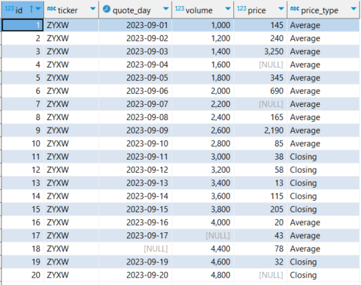
Figure 2. Full sample dataset.
Identifying `null` values
In the case of our dataset, missing values are easily noticeable. However, with a production dataset, it’s not as straightforward. Fortunately, Teradata VantageCloud offers two useful functions: one to filter out rows with missing values in specific columns `TD_GetRowsWithoutMissingValues`, and another to select only those rows, `TD_GetRowsWithMissingValues`.
By leveraging `TD_GetRowsWithoutMissingValues`, we can tally the rows without missing values in the columns that range from `quote_day` to `price_type`, and juxtapose this subset with the complete row count of the dataset.
SELECT count (*) FROM TD_getRowsWithoutMissingValues (

ON analytics_cleaning_demo.cleaning_data_set AS InputTable

USING

TargetColumns ('[quote_day:price_type]')

) AS dt;
This will result in a count of 15.
Given that a quarter of our data has missing values in our specific case, it would be prudent to delve deeper using `TD_GetRowsWithMissingValues`.
SELECT * FROM TD_getRowsWithMissingValues (

ON analytics_cleaning_demo.cleaning_data_set AS InputTable

USING

TargetColumns ('[quote_day:price_type]')

) AS dt;
This returns five columns with missing values, as shown in the following screenshot labeled figure 3. As you can see, the table shows `null` values for `price`, in ids 20, 7, and 4, `volume`, in id 17, and `quote_day`, in id 17.
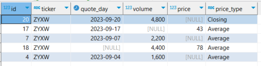
Figure 3. Rows with missing values in the dataset.
Given that price and volume are quantitative, we might opt to fill them using statistical methods, thus retaining those rows. Such choices rely on judgment and context. This is not the case with the row that lacks `quote_day`, so we will directly exclude that row from our analysis.
Having decided, we'll establish a view excluding the row with the missing date, leveraging `TD_GetRowsWithoutMissingValues`.
CREATE VIEW analytics_cleaning_demo.nulls_cleaned AS

SELECT * FROM TD_getRowsWithoutMissingValues (

ON analytics_cleaning_demo.cleaning_data_set AS InputTable

USING

TargetColumns ('quote_day')

) AS dt;
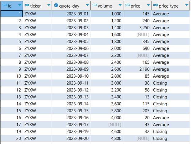
Figure 4. Dataset without NULL values on non-numerical columns from Teradata `TD_GetRowsWithoutMissingValues` function.
Identifying meaningful categorical data
Quantitative data is often aggregated based on categorical data, which should be meaningful for the aggregations to be insightful. If all categorical values are identical, aggregating them is redundant because you would only get the same result that would be returned if you performed the same aggregation across the entire dataset. This could happen if the dataset is a filtered result coming from another dataset. For this example, we are using data obtained by filtering the pricing data of the ticker `ZYXW` from another dataset. Thus, aggregation on the ticker is meaningless in this case.
Conversely, if each row has a unique value, the result of aggregating on said column is just reproducing the dataset. The variability of column values is termed ”cardinality,” and 100% cardinality means that all the values are distinct. When you aggregate on high-cardinality columns, you produce results similar to when you aggregate on columns that only contain distinct values.
Identifying meaningful categorical data in large datasets is not as simple as having a glimpse of the values. This is specifically true regarding cardinality. For this reason, Teradata VantageCloud provides two functions to pinpoint valuable categorical data.
`TD_CategoricalSummary` provides a convenient method to generate an overview of categorical data values. Suppose we're uncertain if our dataset covers multiple tickers or just one. Additionally, suppose we'd like to assess the meaningfulness of aggregating based on `price_type`.
As a first step for this analysis, it’s useful to obtain a summary of the values for these specific categories.
CREATE VIEW analytics_cleaning_demo.category_summaries AS

SELECT * FROM TD_CategoricalSummary (

ON analytics_cleaning_demo.nulls_cleaned AS InputTable

USING

TargetColumns ('ticker','price_type')

) AS dt;
In the code above, we have specified the categorical columns that we intend to summarize. We’ve chosen this parameter according to the needs we’ve assumed above. The results are as follows:
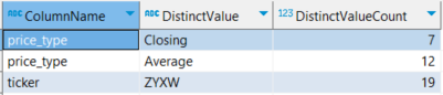
Figure 5. Summary of values of categorical data from Teradata.
Based on this summary, it's clear that our data pertains to a single Ticker. Furthermore, the distribution within `price_type` shows a reasonable level of cardinality. It’s highly unlikely that we could have gleaned such insights through mere visual inspection in a production environment. This type of problem is where in-database analytics functions really stand out.
The function `TD_GetFutileColumns` examines a dataset along with its categorical summary to determine which categories in the summary meet the following criteria:
- Columns with all identical values
- Columns where each value is unique
- Columns where the number of distinct values exceeds a predetermined threshold
First, let’s run the following code, and then evaluate the insights according to our criteria.
SELECT * FROM TD_getFutileColumns(

ON analytics_cleaning_demo.nulls_cleaned AS InputTable PARTITION BY ANY

ON analytics_cleaning_demo.category_summaries AS categorytable DIMENSION

USING

CategoricalSummaryColumn('ColumnName')

ThresholdValue(0.7)

)As dt;
As shown in the following image, the column ticker is futile because it is the same for all records. We also confirm that the `price_type` has a cardinality below our defined threshold of 70% because it didn’t appear in our results.
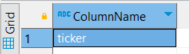
Figure 6. Result of Teradata `TD_GetFutileColumns` function.
We then define a view for further analysis, as shown in the following code sample and the subsequent screenshot of its results:
CREATE VIEW analytics_cleaning_demo.for_analysis AS

SELECT id, quote_day, volume, price, price_type FROM analytics_cleaning_demo.nulls_cleaned;


SELECT * FROM analytics_cleaning_demo.for_analysis;
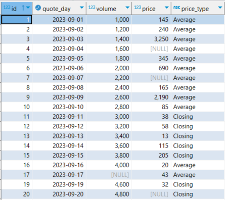
Figure 7. Sample dataset without futile columns.
Fitting missing values
We've prepped our dataset, but there remain some `null` values in the quantitative columns, volume, and price. As previously discussed, rather than discarding these records, we could consider replacing them with a reasonable estimation. Determining the most suitable method to estimate and fill missing values demands domain-specific knowledge, which exceeds the scope of this article, so we cover an example for illustration purposes.
Teradata’s `TD_SimpleImputeFit` function is designed to provide suitable options for fitting out missing values. It provides various customization options to adjust the imputation process, even for textual values. In our case, we'll keep it straightforward: Select the columns to impute and replace the missing values with the median of the available data in those columns.
The result of applying a Teradata fit function, such as `TD_SimpleImputeFit`, to a dataset is known as a fit table— in most cases, nothing more than a statistical description of the data.
Fit tables are widely used to create extra features (shown in columns), based on existing data through a transformation of the existing data. We’ll cover this in an upcoming feature engineering article.
It’s worthwhile to mention that the fit tables resulting from applying `TD_SimpleImputeFit` or the similar function `TD_OutlierFit`, used to identify and fit outlier values, can be used later as part of feature engineering processes, so they’ll often be persisted as tables to avoid recalculations.
CREATE VIEW analytics_cleaning_demo.missing_fitting AS

SELECT * FROM TD_SimpleImputeFit (

ON analytics_cleaning_demo.for_analysis AS InputTable

USING

ColsForStats ('volume','price')

Stats ('median')

) as dt;


SELECT * FROM analytics_cleaning_demo.missing_fitting;

Figure 8. Statistics on quantitative columns computed by Teradata `TD_SimpleImputeFit` function.
With the statistical dimensions defined, the function `TD_SimpleImputeTransform` can take the original dataset and fit the missing values. We define our `for_analysis` table as the input table, and the stats table as the dimension table.
CREATE VIEW analytics_cleaning_demo.missign_fitted AS

SELECT * FROM TD_SimpleImputeTransform (

ON analytics_cleaning_demo.for_analysis AS InputTable

ON analytics_cleaning_demo.missing_fitting AS FitTable DIMENSION

) AS dt;


SELECT * FROM analytics_cleaning_demo.missign_fitted;
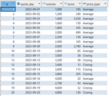
Figure 9. Sample dataset augmented with values computed by the Teradata `TD_SimpleInputTransform` function.
This dataset’s missing values are fitted. Figure 10 shows how the `id` values 4, 7, and 20 are fitted with the median price, 130, and in id 17, and the volume is fitted to the median volume, 2700.
A cleaned dataset, such as the one we produced (but of course much bigger), is ready to serve as a base for ML or generative AI models. However, some feature engineering might be invaluable for such a task—which is why it’s the topic of our next article in this series.
Much more
Teradata VantageCloud comes packed with many more analytics functions for data cleaning and exploration. For example:
- `Pack` and `Unpack`, for transforming single columns into composite columns and vice versa
- `TD_OutlierFilterFit` and `TD_OutlierFilterTransform`, for fitting outliers to smooth out a dataset, and more
Conclusions
Quality data is essential for AI initiatives, and preparing this data is foundational for AI achievements. Teradata VantageCloud offers a suite of robust in-database analytics functions that streamline every stage of your data preparation at scale. In this article, we delved into a selection of these functions, emphasizing data cleaning and exploration phases.
Feedback & questions
We value your insights and perspective! Share your thoughts, feedback, and ideas in the comments below. And, explore the wealth of resources available on the Teradata Developer Portal and Teradata Developer Community.